Pytorch Study Note 1
Prelude
Pytorch is one of the most basic framework machine learning engineers and researchers use these days to model and train and tune. I personally have used Pytorch for almost two years and stumbled upon all the pros and cons in PyTorch code as every researcher does. I think most people learn PyTorch like me, get insights from other people’s work, and adapts to it just by rumbling through the PyTorch documentation. There hasn’t really been a chance for me to slow down and LEARN PyTorch. As I know for all the Machine Learning courses I have taken in the University of Toronto those 4-5 years, there is also no courses focusing on using PyTorch or TensorFlow, they are mostly on the theory, and give you the code and ask you to fill in the blank 😪.
Now, with the time to spend in this pandemic time, I want to take a deeper look at PyTorch, especially how to coordinate between syntaxes and APIs. All the API and knowledge listed below are updated until 2020 PyTorch 1.6.0
You may have noticed that I am showing a very colorful ‘flower’ on my teaser image. What does it have to do with PyTorch? Well, that is actually a Tensor map of white matter in human brain 🧠 made by Alfred Pasieka. Just imagine how complicated a human brain can be – a 3D dimension structure with changing of time – a 4D data, and we hold it with a tensor. I won’t teach you how to make that, even if you follows through all my notes, and feel free to entertain yourself, but this bring us the main character to the table: PyTorch: Tensor.
Table of Content
- Tensor and its initializations
- Operations on tensors (tensor joins, splits, indexing, transformation, and mathematical operations)
- Linear Regression for demo
Tensor and its initializations
1. Tensor
In mathematics, a tensor is an algebraic object that describes a (multilinear) relationship between sets of algebraic objects related to a vector space. Objects that tensors may map between include vectors and scalars, and even other tensors. -Wikipedia

I think you are familiar with the concept of scalar, vector, and matrix, which is usually used to represent data of 1D, 2D, and 3D. Mostly, the Tensor is just another term to explain dimensional data that larger than 3D in Mathematics. You can see it as a meta version of data in any dimension, and that is what it is in PyTorch – a data container compatible for data of all dimensions – even better, it contains the in-built functions for its calculations and attributes, which will be discussed later.
2. Tensor & Variable
Variable is a data type under torch.autograd, and been categorized into Tensor already. The current tensor ‘absorbs’ autograd’s neat property of handling derivatives very conveniently by taking in torch.autograd.Variable entirely. To understand Tensor thoroughly, we can take a look at its simpler version Variable first.
- torch.autograd.Variable
- data: data been encapsulated
- grad: gradient of data
- grad_fn: stands for gradient function, keep track of the methods/operation we used to create the tensor
- required_grad: indicator of if taking derivative is needed
- is_leaf: indicator if current node is a leaf node
grad_fn is very important, which related to how we are going to derive the parameter in the computation graph. This will be elaborated in later chapter
Let’s take a look at Tensor as well:
- torch.tensor
- data: …
- dtype: tensor data type, e.g. torch.FloatTensor, torch.cuda.FloatTensor, data inside usually float32, int64
- shape: keep track of tensor shape in tuple e.g. (m, n, i, j)
- device: tensor device, e.g. CPU/GPU
- required_grad: …
- grad: …
- grad_fn: …
- is_leaf: …
Pretty similar huh?
3. Create a Tensor
3.a. Create directly from data
torch.Tensor(data,
            dtype=None,
            device=None,
            required_grad=False,
            pin_memory=False)
The variable data here can be any common python data types: list or numpy. dtype is the data type same to data by default. The pin_memory when set to True, it loads your samples in the Dataset on CPU and pushes it to the GPU to speed up the host with page-lock memory allocation. For now, we leave it as False as default.
when you create tensor from numpy array, the two data structure will alias in memory, i.e. change of content in numpy array will result changes in tensor and wise-versa
3.b. Create with filled numbers
- We can create a tensor of only 0s inside
torch.zeros(*size, out=None, dtype=None, layout=torch.strided, device=None, required_grad=False)layoutrefers to layout pattern in memory, usually leave as default.outcan take another variable to point to the same tensor location.Similarly,
torch.ones()create a tensor of only 1s,torch.full()create a tensor of any identical number. - Create a tensor of same shape as input, but filled with 0s, 1s or any other numbers
- torch.zeros_like(input, dtype=None, layout=None, device=None, requires_grad=False)
- torch.ones_like()
- torch.full_like()
The names are quite self-explanatory.
- arithmetic sequence
works like
range()in python,torch.arrange(start=0, end, step=1, out=None, dtype=None, layout=torch.strided, device=None, required_grad=False)similarly,
torch.linspace()also gives arithmetic sequence, but it works in closed interval [start, end], whiletorch.arrange()work in semi-closed interval [start, end). Just likelinspace()in numpy - log sequence
torch.logspace(start, end, steps=100, base=10.0 out=None, dtype=None, layout=torch.strided, device=None, required_grad=False)basehere is the base for logistic calculation - diagonal matrix/tensor
torch.eye(n, m=None, out=None, dtype=None, layout=torch.strided, device=None, required_grad=False)nandmare the number of rows and columns for matrix respectively
3.c. Create with probabilities or distributions
- create normal distribution (Gaussian Functions)
This is very commonly used in pytorch.
torch.normal(mean, std, generator=None, out=None)meanis the average;stdis the standard distribution;generatoris of typetorch.Generatora pseudorandom number generator for sampling; andoutis as usual, the output tensormeanandstdboth can be a scalar or a tensor, which bring us four combinations of inputs:- Case 1:
In this case, we have both
meanandstdscalars, the output will be a tensor of size 4, but coming from the same distributiont_normal = torch.normal(0, 1, size=(4,)) - Case 2:
In this case, we have
meanas a scalar butstda tensor, the output will be still a tensor of size 4, but coming from the different distributions all have the same mean valuestd = torch.arange(1, 5, dtype=torch.float) t_normal2 = torch.normal(1, std) - Case 3:
In this case, we have
stdas a scalar butmeana tensor, the output will be still a tensor of size 4, but coming from the different distributions all have the same standard errorsmean = torch.arange(1, 5, dtype=torch.float) t_normal3 = torch.normal(mean, 1) - Case 4:
In this case, we have both
meanandstdtensors, the output will be a tensor of size 4, but coming from the different distribution with different mean and standard errorsmean = torch.arange(1, 5, dtype=torch.float) std = torch.arange(1, 5, dtype=torch.float) t_normal4 = torch.normal(mean, std)
- Case 1:
In this case, we have both
-
Sample from Normal Distributions
torch.randn()andtorch.randn_like()also works with standard normal distribution, returns you an tensor of certain size in that distributiontorch.rand(),rand_like()generates random number from normal distribution on interval [0, 1), whiletorch.randint()andtorch.randint_like()generates on interval [low, high) -
Other Distributions
torch.randperm(n)generates a random permutation of integers from 0 to 0-1, usually used for indexingtorch.bernoulli(input)generates a bernoulli distribution by probability ofinput
Operations on tensors
The operations on tensor is very similar to all the operations on numpy matrix or numpy array, with a few details to notice
1. Basic Operations
1.a. Connecting Tensors
We can connect two tensors by cat or stack, which basically linking two tensors on one dimension. The difference sis that cat stands for concatenate, it joining two tensors on one existing dimension, while stack will create a new dimension and output a tensor that linking the two tensor on this new dimension.
torch.stack(tensors, dim=0, out=None)t = torch.ones((2, 3)) # t = tensor([[1., 1., 1.], # [1., 1., 1.]]) t_stack = torch.stack([t,t,t], dim=0) # stacking on dimension 0 # -> shape = ([3,2,3]) # t_stack = tensor([[[1., 1., 1.], # [1., 1., 1.]], # [[1., 1., 1.], # [1., 1., 1.]], # [[1., 1., 1.], # [1., 1., 1.]]]) t_stack1 = torch.stack([t, t, t], dim=1) # stacking on dimension 1 # -> shape = ([2,3,3]) # t_stack1 = tensor([[[1., 1., 1.], # [1., 1., 1.], # [1., 1., 1.]], # [[1., 1., 1.], # [1., 1., 1.], # [1., 1., 1.]]])-
torch.cat(tensors, dim=0, out=None)t = torch.ones((2, 3)) # t = tensor([[1., 1., 1.], # [1., 1., 1.]]) t_0 = torch.cat([t, t], dim=0) # concatenate by row # t_0 = tensor([[1., 1., 1.], # [1., 1., 1.], # [1., 1., 1.], # [1., 1., 1.]]) t_1 = torch.cat([t, t], dim=1) # concatenate by column # t_1 = tensor([[1., 1., 1., 1., 1., 1.], # [1., 1., 1., 1., 1., 1.]])
1.b. Separating Tensor
We use chunk and split to separate a tensor into many parts. chunk separates a tensor into many equal-size tensors, while split is a more powerful version of chunk, which separates a tensor in to many customized size chunks
torch.chunk(input, chunks, dim=0)t = torch.Tensor([[1,2,3,4,5,6,7],[8,9,10,11,12,13,14]]) # We cut the tensor t of size (2,7) in to three pieces by column, # this will give us (2,3), (2,3) and (2,1) list_of_tensors = torch.chunk(t, dim=1, chunks=3) # list_of_tensors = (tensor([[1,2,3], # [8,9,10]]), # tensor([[4,5,6], # [11,12,13]]), # tensor([[7], # [14]]) # )torch.split(tensor, split_size_or_sections, dim=0)t = torch.Tensor([[1,2,3,4,5,6,7],[8,9,10,11,12,13,14]]) # We cut the tensor t of size (2,7) in to three pieces by column, # this will give us (2,3), (2,2) and (2,2) follows the customized cut list_of_tensors = torch.split(t, [3, 2, 2], dim=1) # list_of_tensors = (tensor([[1,2,3], # [8,9,10]]), # tensor([[4,5], # [11,12]]), # tensor([[6,7], # [13,14]]) # )
1.c. Indexing Tensor
torch.index_select(input, dim, index, out=None)t = torch.randint(0, 9, size=(3, 3)) # generate a random 3x3 matrix from 0-8 # t = tensor([[2, 7, 2], # [4, 3, 8], # [1, 6, 0]]) idx = torch.tensor([0, 2], dtype=torch.long) # index 0-1, notice that the type must be long t_select = torch.index_select(t, dim=1, index=idx) # indexing the 0th column and 1st column # t_select = tensor([[2, 7], # [4, 3], # [1, 6]])torch.masked_select(input, mask, out=None)maskhere is a boolean matrix of the same shape asinputmatrix. A one-dimensional tensor will be returned based on theTrueindex in themask# To select all the values in t that has value >=5 # t = tensor([[2, 7, 2], # [4, 3, 8], # [1, 6, 0]]) mask = t.ge(5) # le(5)-> '<=5', gt(5)-> '>5', lt(5)-> '<5' # mask: # tensor([[False, True, False], # [False, False, True], # [ True, True, False]]) t_select1 = torch.masked_select(t, mask) # t_select1 = tensor([7, 7, 5, 8])
1.d. Transforming Tensor
torch.reshape(input, shape)This function changes the shape ofinputtensor, very commonly used in tensor manipulations. Notice that the matrix afterreshapeand before will share the same addresst = torch.randperm(8) # t = tensor([2,5,1,2,4,3,6,7]) # the -1 is the first dimension back calculated from 8/2/2 automatically by pytorch t_reshape = torch.reshape(t, (-1, 2, 2)) # t_shape = tensor([[[2, 5], # [1, 2]], # [[4, 3], # [6, 7]]])torch.transpose(input, dim0, dim1)Swap the two dimensionsdim0anddim1t = torch.Tensor([[[1,2,3],[4,5,6]],[[7,8,9],[3,2,1]]]) # t = tensor([[[1,2,3], # [4,5,6]], # [[7,8,9], # [3,2,1]]]) t_transpose = torch.transpose(t, dim0=0, dim1=2) # t_transpose = tensor([[[1., 7.], # [4., 3.]], # [[2., 8.], # [5., 2.]], # [[3., 9.], # [6., 1.]]])For 2 dimensional data tensors, we can use
torch.t(input)to transpose the input automatically without predefining the dimensions.torch.squeeze(input, dim=None, out=None)Compress all dimensions that has length of 1t = torch.rand((1, 2, 3, 1)) # t.shape = torch.Size([1, 2, 3, 1]) t_sq = torch.squeeze(t) # t_sq.shape = torch.Size([2, 3]) t_0 = torch.squeeze(t, dim=0) # t_0.shape = torch.Size([2, 3, 1]) t_1 = torch.squeeze(t, dim=1) # t_1.shape = torch.Size([1, 2, 3, 1])while
torch.unsqueeze(input, dim, out=None)is doing the opposite to expand dimension ondim
2. Mathematical Operations
Pytorch supports all kinds of mathematical operations you can think of, including +, -, \(\times\), \(\div\), \(a^x\), \(x^a\), log, and sin/cos
torch.add()
torch.addcdiv()
torch.addcmul()
torch.sub()
torch.div()
torch.mul()

torch.log(input, out=None)
torch.log10(input, out=None)
torch.log2(input, out=None)
torch.exp(input, out=None)
torch.pow()

torch.abs(input, out=None)
torch.acos(input, out=None)
torch.cos(input, out=None)
torch.cosh(input, out=None)
torch.asin(input, out=None)
torch.atan(input, out=None)
torch.atan2(input, out=None)
We will talk a bit more about torch.add(input, other, *, alpha=1, out=None). The alpha here is an extra multiplier works on other, with formula \(out = input + alpha \times other\), where we can simply use torch.add(b, x, alpha=w) to express y=wx+b on linear regression. This is very handy
There are two other similar functions:
-
torch.addcdiv(input, value=1, tensor1, tensor2, out=None)\(out_i = input_i + value \times \frac{tensor1_i}{tensor2_i}\) -
torch.addcmul(input, value=1, tensor1, tensor2, out=None)\(out_i = input_i + value \times tensor1_i \times tensor2_i\)
Which just perfectly bring us the next topic: Linear Regression
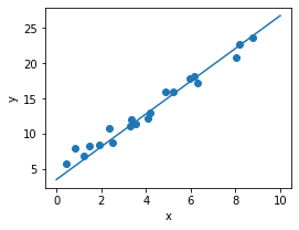
Linear Regression
I will not elaborate how linear regression works, you can check out this link for details, but more on how we implement it in Pytorch
Model: \(y = wx + b\)
Loss: \(MSE = \frac{1}{m}\sum^m_{i=1}(y_i-\tilde{y_i})\)
Gradient Descent for w, b updates:
\[w = w - lr \times w.grad\] \[b = b - lr \times b.grad\]import torch
import numpy as np
import matplotlib.pyplot as plt
# First we randomly generate x, y samples from normal distributions
x = torch.rand(20, 1) * 10 # x ranges from 0 to 10
y = 2 * x + (5 + torch.randn(20, 1))
# set hyperparameters
lr = 0.05 # learning rate
# Construct parameters for gradient descent
w = torch.randn((1), requires_grad=True)
b = torch.zeros((1), requires_grad=True) # Both need to take gradients
# train in 100 iterations
for iteration in range(100):
# Forward propagation
wx = torch.mul(w, x)
y_pred = torch.add(wx, b)
# Calculate loss
loss = (0.5 * (y-y_pred)**2).mean()
# Back propagation
loss.backward()
# Updates gradient
b.data.sub_(lr * b.grad) # this is equivalent to -=
w.data.sub_(lr * w.grad)
# Wipe gradient
w.grad.data.zero_()
b.grad.data.zero_()
print(w.data, b.data)
# tensor([2.3225])
# tensor([3.5149])
# plot linear regression
x_new = np.linspace(0, 10, 100)
y_new = x_new*w.data.tolist()[0]+b.data.tolist()[0]
plt.figure(figsize=(4, 3))
ax = plt.axes()
ax.scatter(x, y)
ax.plot(x_new, y_new)
ax.set_xlabel('x')
ax.set_ylabel('y')
ax.axis('tight')
plt.show()
Summary
This is a small start of ours. It may look tedious to start with, but it becomes crucial when you dive into the ML works later. As it always says:
“The difference between something good and something great is attention to detail.”
Now we have the solid building blocks as our disposal, lets move to the next section: Pytorch Study Note 2 where will talk about PyTorch dynamic computation graph, auto gradient and logistic regression implementations